Motivational Sidenote: This is part of my project in attempting to understand the notion of height (in formal group law theory) in terms of the symmetry of the underlying variety.

Though it may seem disparate, this post is the computation of the Jacobian of a Shiga curve shown to have height 3 properties by Sebastien Thyssen and Hanno van Woerden.

This is only the very first step, the next step is understanding such calculations for Shiga curves with more general roots, for which there may not be a thrice punctured sphere representative.

Thanks to Dami Lee for patiently walking through how to compute the period matrix of this 12-fold cyclic cover of a thrice punctured sphere, and thanks Matthias Weber for showing me how to write the 3-fold cover of a 5-punctured sphere as a 12-fold cyclic cover of a thrice punctured sphere. Most of the figures are either hand-drawn or made using Geogebra. Note that I will sometimes use \(\tau\) to denote \(2 \pi\). All errors are mine and mine alone.

The period matrix of a Riemann surface is defined as \(\int_{\gamma_i} \omega_j\), where \(\omega_1, …, \omega_g\) are a choice of basis of the invariant differentials of the surface, and \(\gamma_1, …, \gamma_{2g}\) are a choice of basis for the Betti \(H_1(S)\).

The Jacobian of a Riemann surface \(S\) is \(\mathbb{C}^g/P\mathbb{Z}\), where \(g\) is the genus of the surface, and \(P\) is the period matrix of \(S\).

We wish to study the Riemann surface cut out by \(y^3 = x^4 -1\), which has roots \((1, -1, i, -i)\) and a ramification point at \(\infty\). Thus, 5 punctures. It is a 3 fold covering because the power of \(y\) is \(3\).

The method of going from a 3-fold cover of the 5 punctured sphere (which Aaron Slipper and I derived) to the cyclic 12-fold cover of the thrice punctured sphere was exposited to me by Matthias Weber, and is as follows. One exhibits an isomorphism between the polynomial \(w^{12} = (v-a)^1 (v-b)^3 (v-c)^8\) and our original polynomial \(y^3 = x^4-1\) The nice thing about thrice punctured spheres is that they are all biholomorphic no matter where the branched points are. So it’s just easier to pick our roots to be 0, 1, and \(\infty\). (This choice also makes it immediately clear that we get a dessin d’enfant!)

We further see that the cover is “cyclically branched” (aka, Dami’s methods apply and I am saved a lot of work), because we get a cyclically branched cover by dividing by a cyclic group, which here is generated by an automorphism of order 12. The automorphism of order 12 is:

\begin{align} x & \mapsto i x \\ y & \mapsto zeta_3 y \end{align}

Note that two triangles make up one copy of the thrice punctured sphere.

I was graciously given unpublished notes of Dami to calculate the Riemannian period matrix via the admissible covers of our thrice-punctured cylcic fellow.

The glory of her method is that to compute \(\int_{\gamma_i} \omega_i\), we simply create, for each \(\omega_1, \omega_2, \omega_3\), a 12-fold cover of the thrice punctured sphere. Each cover has a different set of angles of the triangle and treating the \(\gamma_i\) as vectors on these triangle models gives us their length by representing them as a complex vector.

She defines admissible cone metrics as metrics whose pullback is induced by a holomorphic 1-form, we are exactly trying to understand the basis of holomorphic 1-forms on our Riemann sphere.

An admissible metric on a thrice punctured Riemann sphere is specified by giving 3 angles, the angles of the triangle making up the thrice punctured sphere.

We find this set of angles by using a corollary of Dami’s: if \(\sum a_i = d(n-2)\), and \(a_i = a \cdot d_i (\mod d)\) for all \(d\) and some \(i\) and for some \(a \in \mathbb{Z}\). Then the triangle angles are \((\alpha_i) = (a_i \cdot \frac{\pi}{d})\).

Here, \(d_i = (1, 3, 8)\), and \(d = 12\). So, we look at the following multipliers, [1, 3, 8] [2, 6, 4] [3, 9, 0] [4, 0, 8] [5, 3, 4] [6, 6, 0] [7, 9, 8] [8, 0, 4] [9, 3, 0] [10, 6, 8] [11, 9, 4] and by Dami’s lemma, the admissible ones are the ones which add up to 12 and have no 0 in them. In which case, we get, [1, 3, 8] [2, 6, 4] [5, 3, 4].

First Row

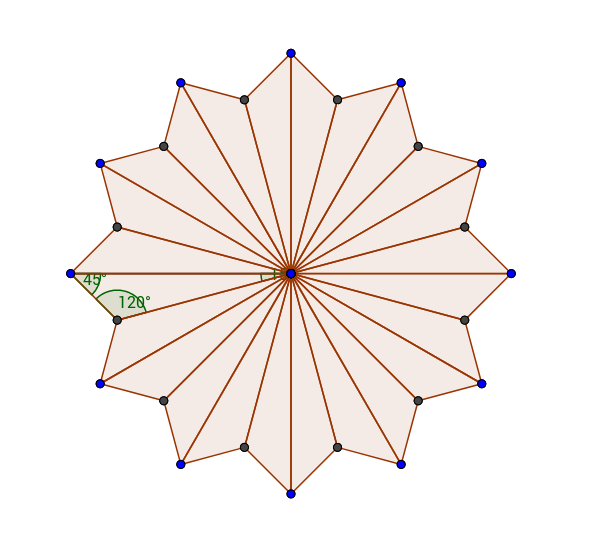
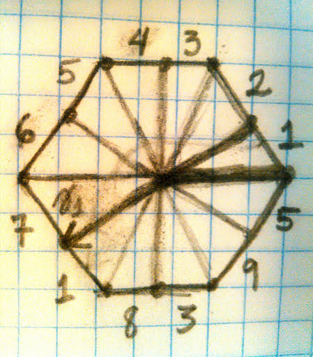
Let us start with the model corresponding to 24 triangles with angles \(\pi/12*(1, 3,8)\), let’s name the distinguished points \((p_1, p_2, p_3)\). Without labels, the figure looks like this:

We can then pick any \(\gamma_j\) combination to parallel edges as long as they satisfy a certain intersection condition. The intersection matrix must have determinant nonzero, we pick the intersection matrix:

\(\begin{pmatrix} A & 0 \\ 0 & A^T \end{pmatrix} \)

Where \(A := \begin{pmatrix} 0 & -1 & 1 \\ 1 & 0 & -1 \\ -1 & 1 & 0 \end{pmatrix}\)

We take the convention that:

• \(\gamma_1\) is associated to the edge labelled 1
• \(\gamma_2\) is associated to the edge labeled 5
• \(\gamma_3\) is associated to the edge labelled 8
• \(\gamma_4\) is associated to the edge labelled 10
• \(\gamma_5\) is associated to the edge labelled 12
• \(\gamma_6\) is associated to the edge labelled 4

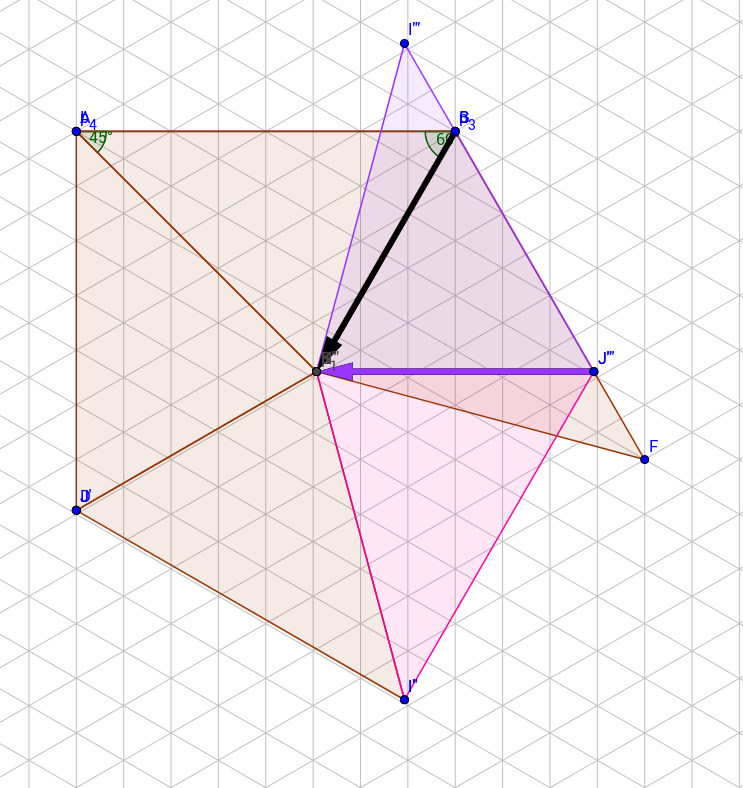
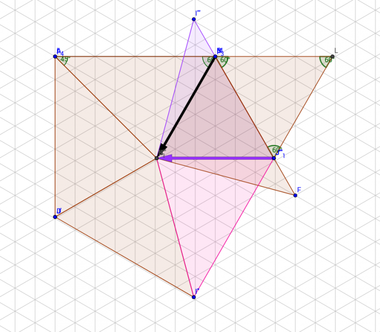
Our surface, with 24 triangles of the appropriate angles, is then the following, the \(v_i\) corresponding to \(\gamma_i\)’s drawn in.

Here, the blue edge dots are \(p_3\), and the black corner dots of the triangles are \(p_2\).

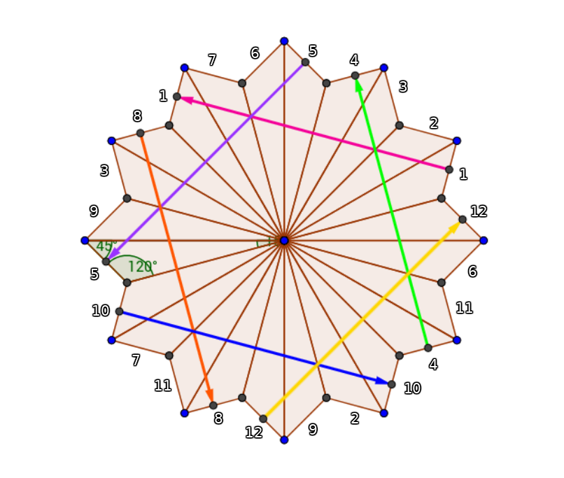
Now, these representations of \(\gamma_1, … \gamma_6\) should be thought of as vectors, \(v_1, …, v_6\). These vectors are the entries in the first row of our period matrix. These are the lengths of \(\gamma_i\) when we integrate over a given 1 form — this 1-form is encoded in the Euclidean representation of our Riemann surface as a 12 fold cover of the thrice punctured sphere.

Now, what is the length of \(\gamma_1\) in terms of the distance between \(p_2\) and \(p_3\), which we will call \(D\).

We see here that the length of \(\gamma_1\) is \((3 + \sqrt{3})\) D where \(D\) is \(d(p_2, p_3)\). Note that the mentioned diagonal of a hexagon is \(\sqrt{3}\)D.

Let us treat \(\gamma_1\) as if it is a straight across real vector (pointing to the left) by rotating our polygon a bit. Thus, \(\int_{\gamma_1} \omega_1 = (-(3 + \sqrt{3}) D, 0)\). Let us write \((3 + \sqrt{3})D\) as \(x\) for short.

Next, we can write down the rest of the vectors, \(\gamma_2, …, \gamma_6\) as rotations of \(\gamma_1\).

Let’s say \(\gamma_2\) is the rotation of \(\gamma_1\) by 120 degrees, then as a vector representation of a complex number, \(\int_{\gamma_2} \omega_1 =(\frac{x}{2}, - \frac{\sqrt(3)}{2} i)\), which is the rotation matrix for \(\theta = 120\) multiplying the vector \(a :=(-x, 0)\). Thinking of \(a\) as a complex number:

So, since \(\gamma_2 \mapsto e^{\tau i/3}a\), then \(\gamma_3 \mapsto e^{2 \tau i/3}a\)
\(\gamma_4 \mapsto e^{3 \tau i/3} a\)
\(\gamma_5 \mapsto e^{4 \tau i /3} a\)
\(\gamma_6 \mapsto e^{5 \tau i/3} a\).

Second Row

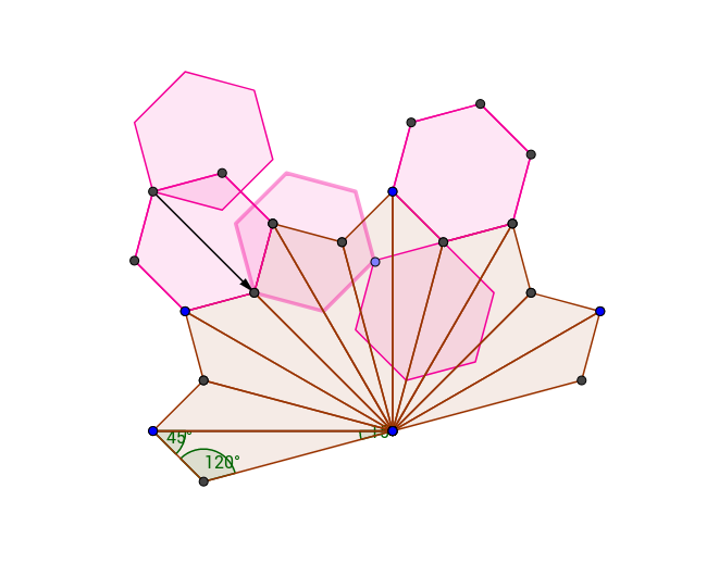
We get the second row of the period matrix from the triangle angles \(\pi/12*(2, 6, 4)\). So when we glue 24 such triangles together (two triangles is one sphere) centered at \(p_1\), we get:

Where the bold line indicates the slit by which the two hexagons are glued together.

We now draw \(\gamma_1\), note that we can draw it as a curvy line, for clarity of thought:

but it is a minimal geodesic, it is more honestly depicted as:

Now we draw in all of the \(\gamma_i\) as curvy lines (though they are actually straight) for clarity, and it is a little more aesthetically pleasing this way I think. These are following the same convention of choices of color and \(\gamma_i\).

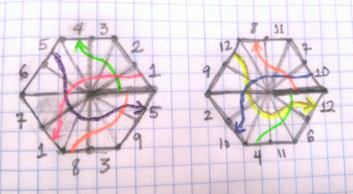
We see that each \(\gamma_j\) is related to \(\gamma_1\) by a rotation of a multiple of \(120\) degrees, that is, \(\tau/3\).

These hexagons have side lengths \(2D\), so the lengths of \(\gamma_i\) are \(2\sqrt{3}D\). Taking the convention that \(\gamma_1\) is always negative facing parallel to the real axis, we get: \(\gamma_1\) will be \(b := -2\sqrt{3}D\). The entries will be: \((b,be^{\tau i/3}, be^{2 \tau i/3}, be^{3 \tau i/3}, be^{4\tau i/3}, be^{5 \tau i/3})\).

That gives us the second row of the period matrix.

Third Row

Last but not least, we treat the case where our 1-form gives us triangle angles \(\pi/12*(5, 3, 4)\), which gives us a fabulous helix-type deal.

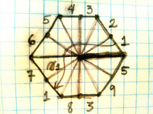
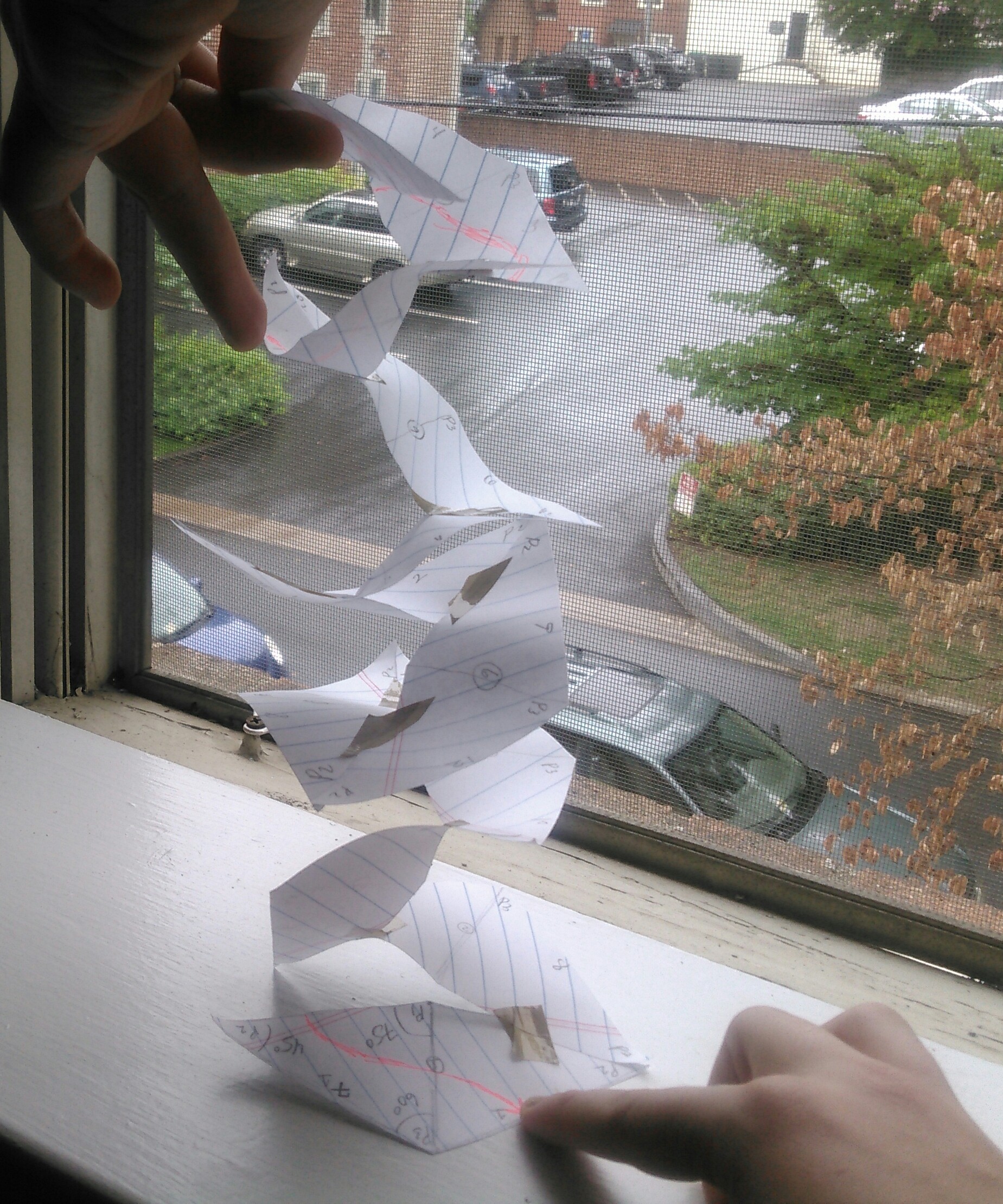
It is easiest to represent in 3D space because unfortunately, we have centered the other drawings around \(p_1\), and in our case, \(p_1\) corresponds to an angle of \(75\) degrees which doesn’t divide 360 evenly until it wraps around itself a few times. Here is my gloriously ill-made 3D paper model:

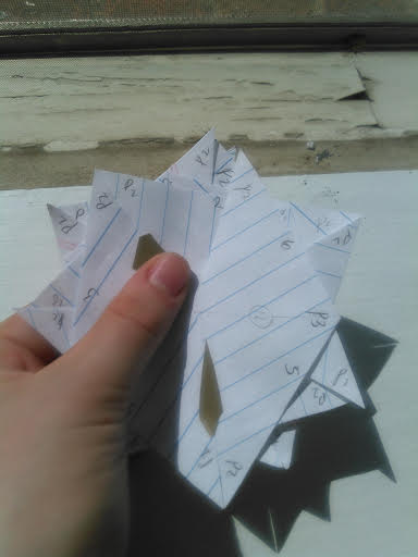
Note that the bottom edge and top edge are in fact identified, though this is not pictured.

So, we start by computing \(\gamma_1\) on this baby, as we usually do. Here, \(\gamma_1\) starts at my left ring finger, and goes to my right pointer finger:

It looks like \(\gamma_1\) as a vector is here \(2d(p_1, p_3)\), since we can pop in and out of \(p_1\) anytime. Here, \(d(p_1, p_3) = \frac{2}{1+ \sqrt{3}}D\) by the rule of sines.

Further, \(\gamma_1\) is related to \(\gamma_2\) by a rotation of \(300\) degrees, that is \(5 \tau/6\) radians.

(We see by reflecting the triangle out as shown below that this angle is 60 degrees.)

In the end, all collected, in complex number form, our period matrix is this glorious beast, let us define

\(a : -(3+\sqrt{3})D\),
\(b := -2\sqrt{3}D\),
\(c := -\frac{4}{1+ \sqrt{3}}D\)

\( \begin{matrix} a & ae^{\tau i/3} &ae^{2\tau i/3} &ae^{3\tau i/3} &ae^{4\tau i/3} &ae^{5\tau i/3} \\ b &b e^{\tau i/3} &b e^{2\tau i/3} & be^{3\tau i/3} & be^{4\tau i/3} &be^{5\tau i/3} \\ c & c e^{5\tau i/6} & c e^{10\tau i/6} & ce^{15\tau i/6} & ce^{20\tau i/6} & ce^{25\tau i/6} \end{matrix}\)