This post is written together with Josh Mundinger. We seek to understand the relations between \(1/2\)’s that appear across mathematics. From the Riemann Hypothesis to the L2 norm, we aim to see the myriad and enticing ways this unfurls; each instance of \(1/2\) connected in an anarchic network of equals. In this blog post, we examine a specific example arising in representation theory: the center of the universal enveloping algebra \(U\mathfrak g\) of a Lie algebra \(\mathfrak g\).

The PBW theorem implies there is an isomorphism of vector spaces \[ sym: \text{Sym}(\mathfrak g)^\mathfrak g \cong Z(U\mathfrak g),\] which on \(\text{Sym}^i\) is given by the symmetrization map \[ sym: x_1x_2\cdots x_i \mapsto \frac{1}{i!} \sum_{\sigma \in S_i} x_{\sigma 1}x_{\sigma 2}\cdots x_{\sigma i}.\]

Note that this is not the identity map because \(Sym\) indicates coinvariants and not invariants of the symmetric group. The symmetrization map is not a ring homomorphism. Duflo showed, however, that by twisting the symmetrization map, one obtains a ring homomorphism. The Chevalley restriction theorem then identifies \(\text{Sym}(\mathfrak g)^\mathfrak g\) with \(\text{Sym}(\mathfrak h)^W\), where \(\mathfrak h\) is a Cartan subalgebra and \(W\) is the Weyl group.

On the other hand, when \(\mathfrak g\) is semisimple, there is another way to understand \(Z(U\mathfrak g)\). The Harish-Chandra isomorphism is a “quantized” version of the Chevalley isomorphism, \[ \text{Sym}(\mathfrak{g})^{\mathfrak{g}} \to \text{Sym}(\mathfrak{h})^{W}. \] It’s called quantized because we are taking taking the universal enveloping algebra, which is adding a parameter deforming the bracket of our Lie algebra (literally a deformation parameter). Then, we get back down to the classical case by taking the associated graded. Harish-Chandra proved that there is an isomorphism \(Z(U\mathfrak g) \cong (U\mathfrak h)^{(W,\cdot)}\). Here \(W\) acts on \(\mathfrak h\) via the \emph{dot action} instead of the usual action: the origin is shifted by \(\rho\), \(1/2\) of the sum of the positive roots of \(\mathfrak g\).

Our quest now leads us to the natural question: are the 1/2 in \(\rho\) and the 1/2 in Duflo’s differential operator the same 1/2?

In the case of \(\mathfrak{sl}_2\), we show via explicit computation that the answer is yes!

In a followup post, we will further see why both arise via a lovely geometric flip and adjustment. The geometric adjustment is by another \(1/2\): a square root of the canonical bundle on a variety.

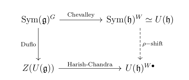
The square with \(\rho\) and Duflo

We investigate the compatibility between three different maps between semi-simple Lie algebras. In particular, we wish to fill in the remaining arrow. We show this commutes explicitly in the case of \(\mathfrak{sl}_2\) by diagram chasing the generator by hand. Let’s go!

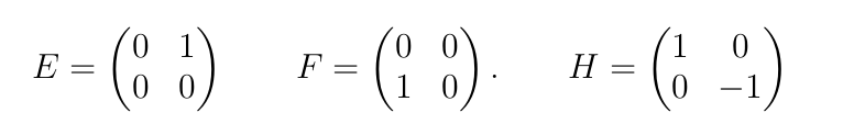
The Lie algebra \(\mathfrak{sl}_2\) has basis \(E,F,H\) with commutation relations \[ [E,F]=H, \qquad [H,E] = 2E, \qquad [H,F] = -2F.\]

The matrices representing \(E, F, H\) are as follows:

The Cartan subalgebra \(\mathfrak h\) is spanned by \(H\), and the Weyl group \(W = \mathbb Z/2\mathbb Z\) acts on \(W\) by \(H \mapsto -H\).

Harish-Chandra

The Harish-Chandra homorphism is defined as follows: there is the Verma module \( M_{\lambda} = U(\mathfrak{sl}_{2})/U(\mathfrak{sl}_{2}) \cdot (E, H - \lambda).\) which we can think of as generated by an element \( 1_{\lambda} \) satisfying \( E1_{\lambda} = 0 \) and \( H1_{\lambda} = \lambda 1_{\lambda} \). We can think of \(\lambda\) as a basis for \(\mathfrak{h}^\ast\) dual to the basis \(H\) of \(\mathfrak{h}\). The module \(M_{\lambda} \) is indecomposable, so \( Z(U \mathfrak{sl}_{2}) \) acts by scalars. The image of \(z \in Z(U\mathfrak{sl}_{2}) \) in \(\mathbb{C}[\mathfrak{h}] = \mathbb{C}[\lambda]\) is the function sending \(\lambda\) to the scalar \( z|_{M_{\lambda}} \).

In the case of \( \mathfrak{sl}_{2} \), We know the center of \(U\mathfrak{sl}_{2} \) is generated by the Casimir operator \(\Omega = EF + FE + \frac{1}{2} H^2 \). That is, \[ Z(U(\mathfrak{sl}_{2})) \simeq \mathbb{C}[\Omega]. \]

Let’s compute the action of Casimir \(\Omega\) on \(1_\lambda\):

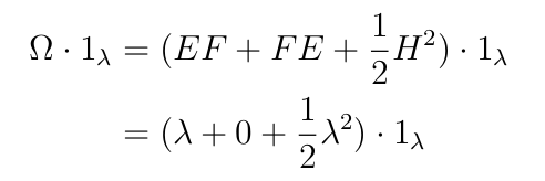
So we have shown that under the Harish-Chandra map,

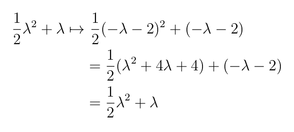
Let’s check that \(\frac{1}{2}\lambda^2 + \lambda\) is invariant under the \(W \bullet\) action. For \(\mathfrak{sl}_2\), we have \([H, E]=2E\), so that the root associated to \(E\) is the function \(\alpha(H) = 2.\) Then, \(\rho\) is \(\frac12\) of the sum of the simple roots, in other words, \(\rho = \frac12 (2) = 1\). The action of \(W \bullet\) sends \(\lambda \mapsto -(\lambda+1)-1 = -\lambda - 2.\)

So we have shown that under the Harish-Chandra map,

Duflo

The Duflo map is defined on the level of vector spaces by acting by a linear operator \(\partial_q: S\mathfrak g \to S\mathfrak g \) followed by the symmetrization map \(S\mathfrak{g} \to U\mathfrak{g} \). We start with expanding a function \(q:\mathfrak{g} \to \mathbb C \) into a power series. A power series expansion of \(q: \mathfrak{g} \to \mathbb{C}\) in terms of the coordinate basis of \(\mathfrak{g} \) is a power series in \(\mathfrak{g}^\ast \). To get \(\partial_q \) from \(q \), we replace each element of \(\mathfrak{g}^\ast \) in the power series with the corresponding partial derivative \(\text{Sym}\mathfrak{g} \to \text{Sym}\mathfrak{g} \). Then, we define the map \(\text{Sym}\mathfrak{g} \to \text{Sym}\mathfrak{g} \) by applying the differential operator to the polynomials that comprise \(\text{Sym}\mathfrak{g} \).

We now define the power series \(q(x) \). Let \(p(x) \) be the function \(\mathfrak g \to \mathbb C \) given by \[ p(x) = \det\left( \frac{sinh(ad(x)/2)}{ad(x)/2}\right) = 1+ \sum_{n=1}^\infty \frac{1}{2^{2n}(2n+1)!}tr(ad(x)^{2n}). \] and let \(q(x) \) be a square root of \(p(x) \) at \(0 \).

We now explicitly express the process of computing the Duflo map with our favorite example \(\mathfrak{sl}_2 \), using the basis \({E,F,H} \). We know the center of \(U\mathfrak{sl}_2 \) is generated by the Casimir operator \(\Omega = EF + FE + \frac{1}{2} H^2 \). Hence, it suffices to compute the action of the Duflo operator on \(\frac{1}{2}H^2 + 2EF \in (S\mathfrak{g})^{\mathfrak g}\). Since the Casimir is quadratic, we only need to know \(q \) up to second order: we have \(q(x) = 1 + \frac{1}{2} \left(\frac{1}{4(6)}tr(ad(x)^2)\right) + O(x^4) = 1 + \frac{1}{48}tr(ad(x)^2) + O(x^4) \). Let’s compute \(tr(ad(x)^2) \) in our coordinates \({E,F,H} \). If \[ x = \begin{pmatrix} a & b \ c & -a \end{pmatrix} = aH + bE + cF ,\] then \(tr(ad(x)^2) = 8a^2 + 8bc \). Hence our differential operator \(\partial_q \) is \[ \partial_q = 1 + \frac{1}{48} (8 \partial_H^2 + 8 \partial_E \partial_F) + h.o.t. = 1 + \frac{1}{6}(\partial_H^2 + \partial_E\partial_F) + h.o.t.\]

Applying this differential operator to \(\frac{1}{2}H^2 + 2 EF \in (\text{Sym}\mathfrak g)^{\mathfrak g}\) gives \[ \partial_q(\frac{1}{2}H^2 + 2EF) = \frac{1}{2}H^2 + 2EF + \frac{1}{6}(1 + 2).\] So applying the symmetrization map gives \[ Duflo(\frac{1}{2}H^2 + 2EF) = \Omega + \frac{1}{2},\] where \(\Omega \) is the Casimir.

Chevalley

Now we compare with the Chevalley isomorphism. The Chevalley map is defined by viewing an element of \(\text{Sym}(\mathfrak g)^{\mathfrak g}\) as an element of \(\mathbb C[\mathfrak g]\) via the Killing form, restricting to \(\mathfrak h\), then again using the Killing form to get an element of \(U\mathfrak h\).

We now express this explicitly in the case of \(\mathfrak{sl}_2\). Under the Killing form, the dual basis to \(\langle H,E,F\rangle\) is \(\langle \frac{1}{8}H, \frac{1}{4}F, \frac{1}{4}E\rangle\). Hence, dualizing, restricting to \(\mathfrak h\), and dualizing again sends \(H\) to \(H\),\(E\) to \(0\), and \(F\) to \(0\), thus sending our element \(\frac{1}{2}H^2 + 2EF \in \text{Sym}(\mathfrak g)^{\mathfrak g}\) to \(\frac{1}{2}H^2\). This is a \(W\)-invariant element of \(U\mathfrak h\) which acts on a highest weight vector \(1_{\lambda}\) by \(\frac{1}{2}\lambda^2\).

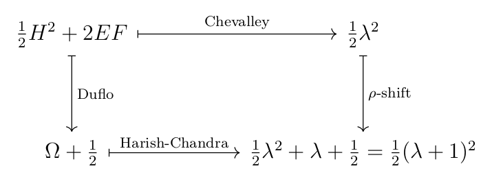
Filling in the Square

We know the center of \( U\mathfrak{sl}_2 \) is generated by the Casimir operator \(\Omega = EF + FE + \frac{1}{2} H^2\). Hence, it suffices to diagram chase this generator through our square to conclude that our square commutes. We showed that the Duflo map sends the symmetrized Casimir operator \(\frac{1}{2}H^2 + 2EF\) in \(\mathfrak{g})^{\mathfrak g} \) to \( \Omega + \frac{1}{2}.\) Further composing with the Harish-Chandra map gives that \(\frac{1}{2}H^2 + 2EF \in (S\mathfrak g)^{\mathfrak g}\) is sent to \(\frac{1}{2}\lambda^2 + \lambda + \frac{1}{2} = \frac{1}{2}\left(\lambda+ 1 \right)^2\).

We now diagram chase the other side. We showed that the Chevalley map sends the symmetrized Casimir operator \(\frac{1}{2}H^2 + 2EF\) to \(\frac{1}{2} \lambda^2\) where \( 1_\lambda \) is the eigenvalue of \(H\). The \(\rho\)-shift map sends \(\lambda\) to \(\lambda + 1\), which sends the image of the Chevalley map \(\frac{1}{2} \lambda^2\) to \(\frac{1}{2} (\lambda + 1)^2\). Therefore, the diagram commutes. We have filled in the square victoriously!