Learning the ultrasonic language of rodents
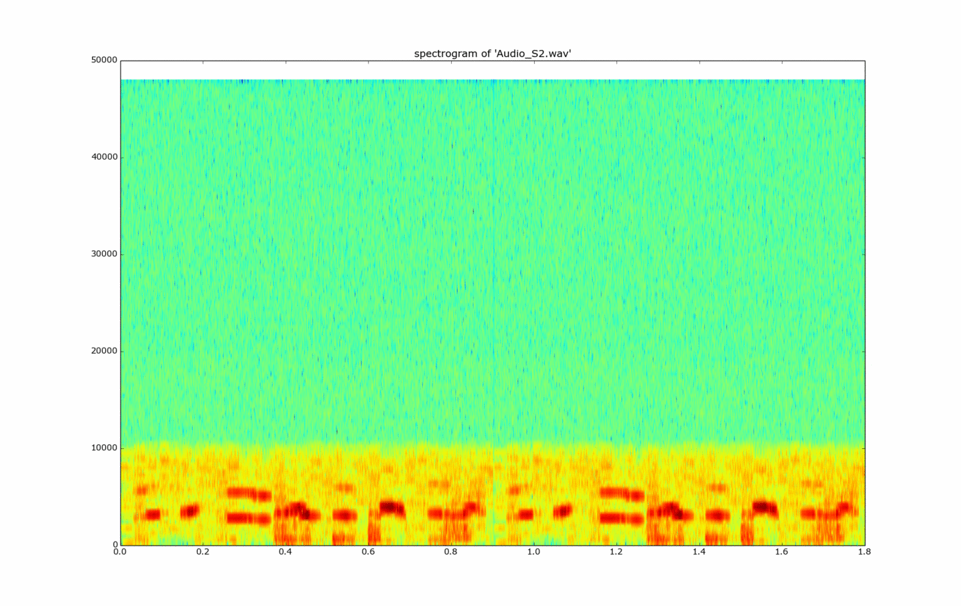
Mice and rats talk to each other constantly, mostly above the range of human hearing. From late 2013 to mid 2014 I worked at Vium on listening in: recording the sounds in a lab cage and teaching a program to pick out the calls and sort them. This post is my write-up from that time, Advances in Mouse Vocalization Research, together with the small scripts and figures that went with it.
Why listen to mice?
When a new drug is tested in mice, you want to catch its side effects on behaviour as early as possible: anxiety, aggression, sexual motivation, development. Listening is a way to watch all of that without opening the cage and breaking the pathogen barrier.
The write-up had three goals:
- FightAlert: notice when mice are fighting, and tell a harmless scuffle from a dangerous fight, so staff get a text message and can step in.
- Produce signals that are useful for research and husbandry in general.
- Use machine learning to sort mouse calls into classes and find out what they are for.
How rodents call
Mice and rats make ultrasonic vocalizations (USVs) by tightening their vocal cords until they work like the plate and hole of a whistle. That gives an almost pure tone. A call we can hear is different: the vocal cords vibrate, which gives a main frequency plus weaker harmonics above it.
A typical call of an adult male mouse is a run of 3–80 pulses. Each pulse lasts 50–300 ms, with rests of about 200 ms in between, so a whole call takes 0.5–30 seconds.
A syllable is one unit of sound, separated from the next by silence. On a spectrogram it is one continuous mark.
What the calls mean
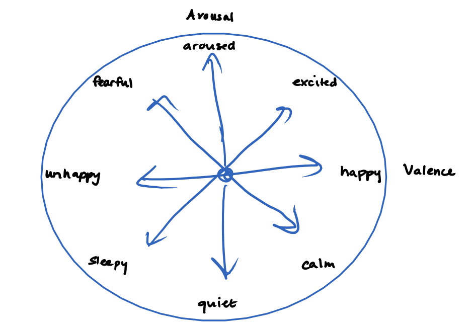
Where a call could sit: how aroused the animal is, and how good or bad it feels.
Richer cages, richer calls. Mice in socially and physically enriched cages make more varied and complex calls than mice alone in single-sex cages.
Females call too. Female mice call while protecting pups, when an intruder enters their cage, while sorting out who is in charge, and during courtship. USVs are not only a male thing. When a new female is put in a resident female’s cage, the resident sniffs her over to learn her rank, sex and reproductive state; unlike two males, two females rarely fight. The resident calls less each time she meets the same partner again, so the drop in calls measures how well she remembers her. This resident–intruder test is a promising way to study how hormones and drugs affect memory.
Pups speed up as they grow. The pulses in pup calls get shorter with age: about 250 ms at 5 days old, about 160 ms at 12 days.
Frequencies of interest in mice
| Frequency | When it happens | Useful for |
|---|---|---|
| 70 kHz | a male courting a female and sniffing her before mounting | husbandry, sexual motivation |
| 40 kHz | mounting (40 kHz calls mixed in with the 70 kHz ones) | husbandry |
| 4 kHz (and 8 kHz) | acute pain | aggression |
A measure of sexual motivation. Male USVs are a well-tested index of sexual motivation, with advantages over watching mating itself: the data are quicker and easier to get, and no partner has to be present. They may even be a purer measure than mating.
Pain calls are audible. In a fight between two males, the subordinate mouse makes dense, layered calls that humans can hear, with a main frequency of 4 kHz and a second one at 8 kHz. The number of these calls tracks how long the mice fight (r = 0.76) and how often one attacks (r = 0.72). They look much the same on a spectrogram whatever the sex of the mouse or the cause of the pain. This is what FightAlert listens for.
Frequencies of interest in rats
Rats have two main adult calls, and they mean opposite things:
- The “22 kHz” call (18–32 kHz, 65–85 dB, 300–4000 ms, barely changing in pitch) comes when a rat expects something unpleasant it cannot escape: a predator, pain, a startle, social defeat. The rat is tense, crouches without moving and breathes hard. Played back, these calls made other rats freeze and avoid; a later study found no drop in avoidance, so what the call is for is still debated.
- The “50 kHz” call (32–96 kHz, 30–50 ms) comes with sex, play between young rats and friendly touch. It is thought to show a good mood.
In short: 22 kHz = bad, 50 kHz = good. Rat pups call at about 40 kHz (80–140 ms, from 4 to 16 days old) when separated from their mother; each call sweeps up or down within 30–65 kHz.
Mice and rats compared
| Rat 22 kHz | Rat 50 kHz | Rat pup | Adult mouse | Mouse pup | |
|---|---|---|---|---|---|
| Frequency | 18–32 kHz | 32–96 kHz | 30–65 kHz | 30–110 kHz (pain: 4 kHz) | 35–110 kHz |
| Duration | 300–4000 ms | 30–50 ms | 80–140 ms | 50–300 ms (pain: 125 ms) | |
| Mood | bad | good | distress |
Unlike rats, adult mice don’t make USVs in unpleasant situations, and their calls have not been shown to carry a good or bad mood.
FightAlert
FightAlert is an alarm for fighting mice: when mice fight, staff get a text message and can react. Pain calls let it tell a harmless scuffle from a dangerous fight. Listening for aggressive calls as well could let staff separate mice before a fight starts.
The first approach: watch the loudness to find the stretches of audio with calls in them, run a short-time Fourier transform (STFT) on those stretches, and run a kernel density estimate (KDE) over the result.
From recording to syllables
A microphone in the cage (an UltraMic) records five minutes at a time, using the monitor script below. The recording is full of other sounds too: moving, gnawing, bumping the cage wall, audible squeaks. Most of that noise is below 30 kHz, but some short snaps land in the ultrasonic band (30–110 kHz).
Every mouse sounds a bit different, their calls change over time, and the background noise changes too. So the program isn’t tuned by hand: it learns from the data, using four thresholds that adapt over time:
- the noise floor of the power spectrum, \(\beta\);
- the noise floor of the amplitude, \(\alpha\);
- the spectral discontinuity;
- the mean frequency of interest.
Step 0: throw out empty files. Normalize the recording, then compare its power spectrum with the expected noise. If nothing rises above it, there are no candidate calls and the file is skipped.
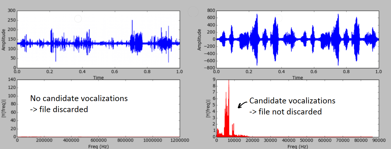
Step 1: find the noise floor. For the files that are kept, the noise floor is the median amplitude plus one standard deviation.
Step 2: cut out the candidates (“snibbets”). A snibbet starts when the amplitude rises above the noise floor and ends when it drops back below. The program starts 3 time bins early so it catches the whole call. It also finds the peaks and splits the recording at each one, to measure how jumpy the audio is.
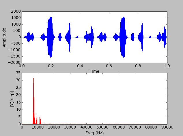
Step 3: decide which candidates are really calls. Following Holy and Guo (2005), the program tracks three things over time, each smoothed with a 10 ms median filter:
- the mean frequency;
- the spectral purity, how much of the power sits in the single loudest frequency: \(\frac{\max(\text{snibbet})}{\sum_i \text{snibbet}_i}\) where a snibbet here is the power spectrum of a piece of the recording;
- the spectral discontinuity, how much the spread of power across frequencies jumps from one time bin to the next: \(\delta_i = \min_{\Delta j} \sum_j \left\lvert \hat{p}_{i+1}(f_{j+\Delta j}) - \hat{p}_i(f_j) \right\rvert\) where \(\hat{p}_i(f_j)\) is the normalized power at frequency \(f_j\) in time bin \(i\).
A candidate counts as a call if:
| Test | Threshold |
|---|---|
| it lasts | more than 5 ms |
| mean frequency | above 35 kHz |
| spectral purity | above 0.25 |
| spectral discontinuity \(\delta\) | below 1 |
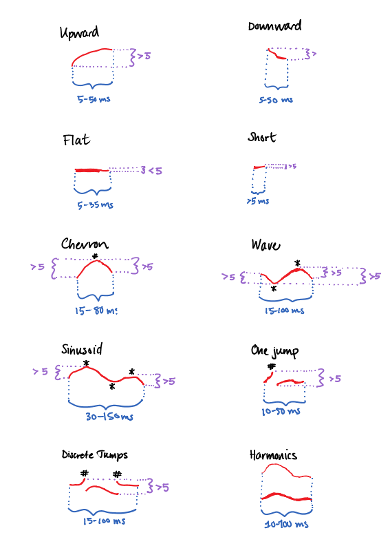
Step 4: sort the calls. Each syllable is described by its starting frequency, ending frequency, the frequency with the most energy, how much its pitch changes, and how long it lasts. There were two ways to sort them:
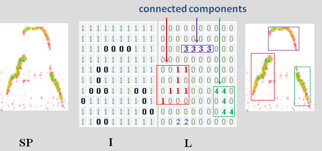
- Unstructured: let the data decide, using MUSIC together with component analysis: find each call’s shape as a connected component of the spectrogram, then look for clusters. The results are stored so they can be mined later, to find structure nobody has named yet.
- Structured: sort calls into the syllable types already known from the literature.
Ideas for later
Hearing as a stress test. How much a mouse freezes and avoids when tones are played to it measures how sensitive its hearing is, and that looks promising as a way to measure stress without touching the animal.
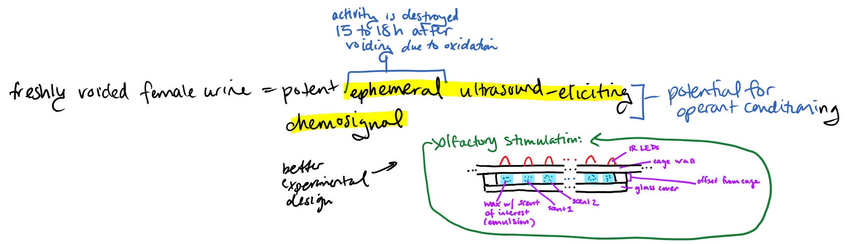
Getting mice to call. Fresh urine from a female mouse is a strong trigger for male calls. Its effect wears off 15–18 hours after it is voided, because the major urinary proteins that carry the signal oxidize. Female urine also makes males release luteinizing hormone (Maruniak and Bronson, 1976), encourages mating and reduces aggression between males (Mugford and Nowell, 1971). Because it wears off, it is a trigger you can control, so I sketched a small device for fresh olfactory stimulation.
The scripts
Three small scripts from the project. They are Python 2, as it was in 2014.
Record five minutes of audio, named by the time it started (monitor.sh):
#!/bin/sh
# Catherine Ray
# Script to record 5 minute audio  [indexed by time] stored in /songs

# Establish current time
DAY=$(date +%d) # set variable $DAY for day
MO=$(date +%m)  # set variable $MO for month
YR=$(date +%y)  # set variable $YR for year (2 digits)
H=$(date +%H)   # set variable $H for hour (24 hour)
M=$(date +%M)   # set variable $M for minute
NOW=$(date)     # sets date / time variable $NOW

arecord -d300 -D plughw:1,0 sea.mousera.net:/usr/local/www/xbox/$YR$MO$DAY-$H$M.wav  # records audio for 300s=5min
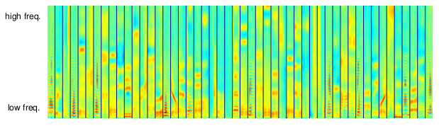
Draw a spectrogram of a recording; this made the picture at the top (spectrogram.py):
"""Generate a Spectrogram image for a given WAV audio sample.

A spectrogram, or sonogram, is a visual representation of the spectrum
of frequencies in a sound.  Horizontal axis represents time, Vertical axis
represents frequency, and color represents amplitude.
"""


import os
import wave
import sys
import pylab


def graph_spectrogram(wav_file):
    sound_info, frame_rate = get_wav_info(wav_file)
    pylab.figure(num=None, figsize=(19, 12))
    pylab.subplot(111)
    pylab.title('spectrogram of %r' % wav_file)
    pylab.specgram(sound_info, Fs=frame_rate)
    pylab.savefig('spectrogram.png')


def get_wav_info(wav_file):
    wav = wave.open(wav_file, 'r')
    frames = wav.readframes(-1)
    sound_info = pylab.fromstring(frames, 'Int16')
    frame_rate = wav.getframerate()
    wav.close()
    return sound_info, frame_rate


if __name__ == '__main__':
    wav_file = sys.argv[1]
    graph_spectrogram(wav_file)
Plot the amplitude and the frequency spectrum, the first try at steps 0 and 1; this made the two-panel plots above (frequency_spectrum.py):
from numpy.fft import *
from numpy import median, std, linspace, pi
from pylab import plot, show, title, xlabel, ylabel, subplot
from scipy import fft, arange
import numpy
import scipy
import sys
import scipy.io.wavfile


def wav_to_arr(wavefile):

    # get relevant info about file
    fs, sig = scipy.io.wavfile.read(f)
    framerate = fs
    nframes = len(sig)
    params = [framerate, nframes]

    return sig, params


def plot_signal(wav_arr):
    """
    2 Plots: (0) amplitude vs. time & (1) amplitude spectrum.
    """
    y = wav_arr
    Fs = len(y);  # sampling rate
    Ts = 1.0/Fs; # sampling interval
    t = arange(0,1,Ts) # time vector

    subplot(2,1,1)
    plot(t,y)
    xlabel('Time')
    ylabel('Amplitude')
    subplot(2,1,2)
    plotSpectrum(y,Fs)
    show()


def plotSpectrum(y,Fs):
    """
    Plots a Single-Sided Amplitude Spectrum of y(t)
    """
    n = len(y) # length of the signal
    k = arange(n)
    T = n/Fs
    frq = k/T # two sides frequency range
    frq = frq[range(n/2)] # one side frequency range

    Y = fft(y)/n # fft computing and normalization
    Y = Y[range(n/2)]
    Y = abs(Y) #single-sided

    print median(Y) + std(Y)
    #print [y for y in Y if y > median(Y)+std(Y)]

    plot(frq,abs(Y),'r') # plotting the spectrum
    xlabel('Freq (Hz)')
    ylabel('|Y(freq)|')


def extract_snibbets(wav_arr):
    for frame in range(0,len(wav_arr)):
        #if frame > noise_floor(wav_arr):
        if frame > 6:
            snibbet.append(frame)
        else:
            snibbet.append("0") #placeholder

#def syllable():


#def noise_floor(n): #adaptive noise floor

if __name__=="__main__":
    f = "t.wav"
    #f = sys.argv[1]
    #convert *.wav to array
    wav_arr, params = wav_to_arr(f)
    plot_signal(wav_arr)
Further reading
- Timothy E. Holy and Zhongsheng Guo, Ultrasonic Songs of Male Mice, PLoS Biology 3(12), 2005.
- Christine V. Portfors, Types and Functions of Ultrasonic Vocalizations in Laboratory Rats and Mice, JAALAS 46(1), 2007.
- Gustavo Arriaga, Eric P. Zhou and Erich D. Jarvis, Of Mice, Birds, and Men: The Mouse Ultrasonic Song System Has Some Features Similar to Humans and Song-Learning Birds, PLoS ONE 7(10), 2012.
- Jesin Zakaria, Sarah Rotschafer, Abdullah Mueen, Khaleel Razak and Eamonn Keogh, Mining Massive Archives of Mice Sounds with Symbolized Representations, SDM 2012. An entertaining one: they map mouse syllables to Farsi numerals, which fit as well as anything else.